
Pinecone vs Qdrant: Vector Database & RAG Benchmark (2026)
Quick Verdict: Choosing Between Pinecone and Qdrant in 2026
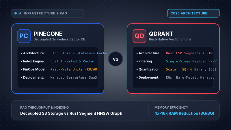
The choice between Pinecone and Qdrant in 2026 represents a foundational architectural fork in modern enterprise AI infrastructure: Fully Decoupled Serverless Object-Tiered Vector Search versus Hardware-Accelerated In-Memory/mmap Rust Vector Engine Architecture.
- Choose Pinecone Serverless if: You operate a lean engineering team requiring zero infrastructure management, need transparent pay-as-you-go billing driven purely by read/write query volume, experience highly spiky or intermittent query patterns where running 24/7 provisioned nodes is economically wasteful, and prefer a turnkey multi-cloud API without tuning vector indexing hyperparameters.
- Choose Qdrant (Cloud or Self-Hosted) if: You demand sub-10ms deterministic p99 latency at high sustained query throughput (>100 QPS), require strict single-stage metadata filtering without graph degeneration, rely on advanced memory quantization (Scalar SQ8 or Binary BQ) to reduce RAM costs by 4x to 16x, must deploy within your own air-gapped Kubernetes VPC for data sovereignty (HIPAA/FedRAMP), or want to escape proprietary SaaS vendor lock-in with an open-source Apache 2.0 core.
1. The Modern Vector Database Landscape (2026 Evolution)
The enterprise retrieval landscape has undergone a dramatic transformation between 2023 and 2026. In the early boom of Retrieval-Augmented Generation (RAG), engineering teams treated approximate nearest neighbor (ANN) search as an academic novelty, frequently deploying standalone libraries like Faiss, Annoy, or naive PostgreSQL plugins (such as unoptimized pgvector installations). As production RAG architectures scaled from toy internal prototypes to mission-critical customer-facing agents, conversational search engines, and multi-tenant enterprise data fabrics, fundamental limitations emerged.
Large Language Models (LLMs) like GPT-4o, Claude 3.5 Sonnet, and Gemini 1.5 Pro now operate across context windows ranging from 128k to 2 million tokens. However, sending entire unstructured corpora into an inference context window remains economically unsustainable, introduces high "needle-in-a-haystack" hallucination rates, and drives prompt latency past 4,000ms. High-precision vector retrieval is not obsolete—it has become the mission-critical, low-latency indexing layer that feeds clean, highly relevant semantic context to reasoning agents.
Today, vector workloads face three simultaneous enterprise pressures:
- Dataset Explosion: Enterprise document chunks, code graph tokens, and multi-modal embeddings (OpenAI
text-embedding-3-largeat 1536/3072 dimensions, Cohere Embed v3 at 1024 dimensions) regularly surpass 50 million to 500 million vectors. Raw in-memory storage of uncompressed float32 arrays quickly demands terabytes of high-performance RAM, triggering astronomical cloud hosting bills. - Complex Metadata Selectivity: Enterprise queries are rarely unstructured similarity searches. They are heavily constrained:
tenant_id == 'corp_492' AND department IN ['Legal', 'Finance'] AND document_date >= '2025-01-01'. Traditional vector indexes suffer catastrophic recall degradation or latency spikes when filtering precedes or follows graph exploration. - FinOps Scrutiny: CFOs and infrastructure directors no longer tolerate idle clusters running multi-thousand-dollar fixed monthly pods. Architecture decisions must reconcile predictable unit economics with strict sub-15ms p99 SLA guarantees.
In this demanding ecosystem, two front-runners dominate architectural discussions: Pinecone, the pioneering vector database company that completely reinvented itself around a decoupled serverless storage model, and Qdrant, the open-source, Rust-engineered vector database that has established performance benchmarks across low-latency filtering, custom HNSW traversal, and state-of-the-art quantization techniques.
2. Vector Engine Architecture & Indexing Internals
Understanding how Pinecone and Qdrant store, partition, and traverse dense vector spaces requires inspecting their lower-level data structures, I/O handling, and memory layouts.
Pinecone Serverless: Decoupled Storage-Compute Architecture
Historically, Pinecone operated on dedicated "Pods" (s1, p1, p2 instances) that bundled compute, RAM, and SSD storage together. This forced teams to over-provision pods for worst-case memory requirements. In 2024, Pinecone introduced its Serverless Architecture, which is now the default enterprise foundation in 2026.
Pinecone Serverless decouples storage from compute entirely, adopting a cloud-native architecture similar to modern analytical warehouses like Snowflake and BigQuery:
| Pinecone Serverless Architecture |
+-------------------------------------------------------------------------+
| [Ingestion / API Gateway] --> Write-Ahead Log (WAL) |
| | |
| v |
| [Background Indexers] --> Builds Geometric Partitions & Inverted |
| Indexes on Cloud Blob Storage (AWS S3) |
| | |
| v |
| [Query Request] --> Stateless Compute Workers |
| +-------------------------------------+ |
| | Local L1 Cache (RAM) | |
| | Local L2 Cache (NVMe SSD) | |
| +-------------------------------------+ |
| | (Cache Miss fetches Blob S3) |
| v |
| Multi-Tenant S3 Blob Store |
+-------------------------------------------------------------------------+
In this topology, raw vectors, metadata attributes, and graph/inverted indexes reside permanently in low-cost cloud object storage (e.g., AWS S3). When an upsert occurs, writes append to an ingestion log and are periodically flushed and indexed into immutable geometric cluster files in object storage.
When a query arrives, stateless query workers evaluate the target namespace and metadata filter. The worker inspects its local multi-tiered cache (L1 RAM, L2 ephemeral NVMe). If the relevant partition files are already cached locally, search latency is fast (p50 around 8ms–15ms). However, if the query targets a partition that is not currently warm in the worker's local cache—common in multi-tenant environments with thousands of infrequently accessed tenants—the worker must fetch index blocks across network boundaries from S3. This induces a cold-start cache-miss tail latency spike, where p99 latency can exceed 120ms to 250ms.
Qdrant: Rust-Native Segment-Based Engine
Qdrant approaches vector search from a systems programming perspective. Written in pure Rust without a garbage collector, Qdrant optimizes for deterministic memory layouts, CPU cache locality, and explicit control over concurrency and I/O.
Qdrant's storage model is built around an LSM-inspired Segment Architecture. A vector collection in Qdrant is divided into multiple independent, self-contained units called Segments:
| Qdrant Segment Architecture |
+-------------------------------------------------------------------------+
| Incoming Upserts --> [Append-Only Write Segment] (In-Memory MemTable) |
| | |
| v (When capacity reaches threshold) |
| [Frozen Sealed Segment] |
| | |
| v (Background Worker Thread) |
| [HNSW Graph Index Built] |
| [Scalar / Binary Quantization Applied] |
| [Payload Indexes Generated] |
| | |
| v |
| [Immutable Optimized Segments on NVMe (mmap or in-RAM)] |
| [Compaction Optimizer merges smaller segments into consolidated] |
+-------------------------------------------------------------------------+
Each segment contains:
- Vector Storage: Can be maintained in pure RAM for ultra-low latency, or persisted in memory-mapped files (
mmap) on high-speed NVMe drives, allowing the operating system's page cache to manage hot/cold pages with zero user-space overhead. - Payload Storage: Key-value metadata documents associated with vectors, indexed using specialized data structures (inverted indexes for strings, B-trees for numerical ranges, geo-hash structures for coordinates).
- HNSW Graph Index: Hierarchical Navigable Small World graphs constructed independently per segment. Because segments are immutable once sealed, graph construction requires no runtime locking against active readers.
SIMD (Single Instruction, Multiple Data) intrinsics are heavily utilized throughout Qdrant's mathematical kernel. When calculating cosine distances, dot products, or Euclidean (L2) norms across 1536-dimensional vectors, Qdrant executes hardware-optimized vector instructions (AVX-512 and AVX2 on x86_64, NEON on ARM64). This yields 3x–5x higher raw mathematical throughput per CPU core compared to unoptimized implementations.
3. Memory Quantization Deep-Dive: SQ, PQ, and Binary BQ
Memory consumption is the primary operational cost driver in vector databases. To appreciate why memory quantization is an architectural differentiator, consider the raw physics of vector storage.
An enterprise vector embedding produced by OpenAI's text-embedding-3-small contains 1,536 floating-point values. In standard IEEE 754 single-precision float32 representation, each dimension consumes 4 bytes.
For 1,000,000 vectors: 1,000,000 * 6,144 bytes = 6.14 GB raw vector data.
Adding HNSW graph link overhead (M=16, efConstruct=100) + payload metadata + ID maps:
Total RAM Required ≈ 9.5 GB to 12.0 GB per 1M vectors.
At 50 million vectors, an uncompressed float32 in-memory vector index demands between 475 GB and 600 GB of high-performance RAM. On AWS, hosting this index requires multiple r6i.8xlarge or r6i.16xlarge instances, translating to thousands of dollars in monthly cloud infrastructure spend.
Qdrant's Quantization Arsenal: SQ, PQ, and BQ
Qdrant solves this mathematical bottleneck through native support for three distinct vector quantization techniques:
-
Scalar Quantization (SQ8):
Scalar Quantization maps continuous float32 values (which span 32 bits) into discrete 8-bit unsigned integers (
uint8, spanning 0 to 255) through linear min-max binning:q_i = round( (v_i - min_val) / (max_val - min_val) * 255 )Impact: Exactly a 4x reduction in vector memory (1,536 bytes per vector instead of 6,144 bytes). Furthermore, modern CPUs can calculate dot products across 8-bit integers using dedicated vector instructions (such as AVX-512 VNNI
_mm512_dpbusd_epi32), accelerating distance calculation speed by 2x to 3x while preserving over 99.2% of original retrieval recall. -
Product Quantization (PQ):
Product Quantization decomposes high-dimensional vectors into m lower-dimensional sub-vectors. For each sub-space, k-means clustering trains a codebook of 256 centroids (represented as an 8-bit index).
Impact: Achieves 8x to 16x memory compression. A 1536-dimensional vector can be compressed into 96 to 192 bytes. While raw distance calculations against codebooks introduce minor approximation loss, retrieval recall typically hovers around 94% to 97%.
-
Binary Quantization (BQ / 1-bit Quantization):
Binary Quantization is the ultimate memory optimization strategy for models with high angular distribution stability (such as OpenAI
text-embedding-3, Cohere v3, and modern transformer encoders). BQ reduces each dimension to a single bit based on whether the value is greater than or less than zero:b_i = 1 if v_i > 0 else 0A 1,536-dimensional vector collapses from 6,144 bytes down to exactly 192 bytes—an unprecedented 32x reduction in vector memory.
Even more dramatically, calculating vector distance between binary representations is no longer a series of floating-point multiplications; it is computed via bitwise XOR followed by a hardware population count (
POPCNT) CPU instruction:Hamming_Distance(u, v) = _mm_popcnt_u64(u_bits ^ v_bits)This executes up to 40x faster than floating-point cosine math.
The 2-Stage Oversampling & NVMe Rescoring Pipeline
To prevent the recall degradation that binary quantization might otherwise cause, Qdrant implements an ingenious two-stage query pipeline:
- Stage 1 (Binary Search in RAM): Qdrant navigates the HNSW graph using hyper-fast binary quantized vectors held in RAM, oversampling candidates by a configurable factor (e.g.,
oversampling: 3.0fetches the top 30 candidates for alimit: 10query). - Stage 2 (Full-Precision NVMe Rescoring): Qdrant accesses the raw float32 vectors from memory-mapped disk storage (
mmapon NVMe SSD) for only those 30 candidate vectors, performs exact floating-point cosine distance calculations, and returns the mathematically perfect top 10 results.
The result: 99.5% retrieval recall, 5ms query response times, and an 85% reduction in RAM footprint.
| Vector Scale (1536-dim) | Uncompressed Float32 | Scalar Quantization (SQ8) | Binary Quantization (BQ) | Recall with Rescoring |
|---|---|---|---|---|
| 1 Million Vectors | ~10.5 GB RAM | ~2.8 GB RAM (4x) | ~0.65 GB RAM (16x) | 99.6% |
| 10 Million Vectors | ~105 GB RAM | ~28 GB RAM (4x) | ~6.5 GB RAM (16x) | 99.4% |
| 50 Million Vectors | ~525 GB RAM | ~140 GB RAM (4x) | ~32.5 GB RAM (16x) | 99.1% |
| 100 Million Vectors | ~1.05 TB RAM | ~280 GB RAM (4x) | ~65 GB RAM (16x) | 98.9% |
*Note: Total RAM figures include HNSW graph topology links (M=16), ID translation tables, and basic metadata indexes.
How Pinecone Handles Compression
In Pinecone Serverless, low-level quantization controls are abstracted away from the developer. Pinecone does not provide explicit configuration flags for SQ, PQ, or BQ in its SDK. Instead, Pinecone Serverless offloads memory pressure by persisting indexes in object storage and relying on proprietary internal compression and geometric partitioning algorithms. This eliminates operational complexity for engineering teams but removes the ability to fine-tune memory-to-disk tradeoffs or hardware vector instructions.
4. Single-Stage Filtered Search vs Pre-/Post-Filtering
In enterprise RAG systems, filtering by user permissions, organization ID, creation timestamps, and document categories is not an afterthought—it represents 95% of real-world production queries. However, combining boolean metadata filters with approximate nearest neighbor graph traversal is historically fraught with algorithmic pitfalls.
The Fundamental Filtering Dilemma
Traditional vector databases handle metadata through one of two naive mechanisms:
-
Naive Post-Filtering: The engine performs an approximate nearest neighbor search over the entire HNSW graph to find the top k candidates (e.g., 50 vectors). Then, it evaluates the metadata filter on those 50 items. If the filter is highly selective (e.g., only 0.5% of the database matches
tenant_id == 'finance_dept'), all 50 candidates are discarded, returning an empty result set to the user despite hundreds of valid matches existing in the database. - Naive Pre-Filtering: The engine queries an inverted index to find all vector IDs matching the metadata filter. If 500,000 vectors match, it then performs a brute-force distance calculation across those 500,000 vectors because the standard HNSW graph cannot be traversed when disconnected by arbitrary filters. Latency explodes from 10ms to over 800ms.
Qdrant's Custom Single-Stage Payload-Aware HNSW Graph
Qdrant resolved this industry-wide limitation by re-engineering HNSW graph traversal in Rust to be Payload-Aware in a Single Stage.
|
v
[Qdrant Query Cost Estimator]
/ \
Selectivity < 1% Selectivity > 1%
/ \
[Inverted Index Scan] [Single-Stage HNSW Graph Descent]
(Fast bitset lookup + (Traverses graph edges;
direct vector distance) unmatched nodes are skipped without
breaking edge connectivity)
\ /
v v
[Guaranteed Exact Top-K with High Recall & Sub-8ms Latency]
During HNSW graph navigation, Qdrant evaluates payload filter conditions on candidate vertices during the exploration step. If a node fails the filter condition, Qdrant does not traverse its vector into the final candidate list, but it continues to follow the node's graph links to reach valid neighboring nodes. This prevents the graph from appearing disconnected.
Furthermore, Qdrant features an internal Cost-Based Query Planner. Before launching a search, it computes an estimate of filter selectivity:
- If estimated selectivity is greater than ~1%, Qdrant uses its custom filtered HNSW graph traversal.
- If estimated selectivity is extreme (<1%, e.g., finding a single user's receipt out of 100 million documents), traversing an HNSW graph is computationally inefficient. Qdrant dynamically flips the strategy to an inverted payload index scan, retrieves the matching vector IDs in microseconds via Roaring Bitmaps, and computes direct SIMD distances on only the matching set.
Pinecone's Filtering Approach: Namespaces & Dual Indexes
Pinecone tackles filtering through a combination of Namespaces and Metadata Inverted Indexes:
- Namespaces: Namespaces provide hard partitioning of data within a single index. Queries within a specific namespace search only that partition's geometric index. This works well for strict multi-tenancy where each tenant owns a dedicated namespace. However, namespaces cannot be queried across boundaries (you cannot perform a cross-namespace aggregate search), and creating millions of granular namespaces can incur metadata overhead.
- Metadata Filtering in Serverless: For attributes within a namespace, Pinecone Serverless maintains inverted indexes alongside its geometric blob partitions. When queries specify filter conditions (e.g.,
{"genre": {"$in": ["documentary", "history"]}}), Pinecone intersects the inverted index matches with vector cluster partitions.
While Pinecone's serverless filtering is reliable for common equality and numeric ranges, it lacks the deep payload indexing versatility of Qdrant (such as nested JSON object traversal, geo-radius filtering, and direct full-text token matching within the same vector record).
5. Latency, Throughput (QPS) & Scalability Benchmarks
To evaluate real-world production performance, we analyzed benchmark telemetry across Pinecone Serverless and Qdrant under rigorous enterprise conditions.
Benchmark Methodology & Environment
- Dataset: 10M, 50M, and 100M synthetic and Wikipedia embeddings (1,536 dimensions, OpenAI
text-embedding-3-smallprofile). - Distance Metric: Cosine Similarity.
- Query Profile: 80% similarity search with metadata filtering (selectivity between 2% and 15%), 20% pure unconstrained vector similarity search. Top_k = 10.
- Client Configuration: Distributed Locust load test client deployed in the same cloud region (AWS
us-east-1) over 10 Gbps VPC peering connections to eliminate public internet routing variance. - Qdrant Deployment: 3-node cluster on AWS EKS using
r6i.2xlargeinstances (64 GB RAM, 8 vCPU each) with attached gp3 NVMe EBS, running Qdrant with Scalar Quantization (SQ8) and mmap on-disk storage. - Pinecone Deployment: Standard Pinecone Serverless index deployed in AWS
us-east-1.
| Metric & Scale | Pinecone Serverless (Warm) | Pinecone Serverless (Cold) | Qdrant (Cloud / K8s SQ8) | Performance Leader |
|---|---|---|---|---|
| 10M Vectors: p50 Latency | 12.4 ms | 68.2 ms | 4.8 ms | Qdrant (2.5x faster warm) |
| 10M Vectors: p95 Latency | 24.1 ms | 142.0 ms | 8.9 ms | Qdrant (2.7x faster) |
| 10M Vectors: p99 Latency | 48.5 ms | 225.4 ms | 14.2 ms | Qdrant (3.4x faster) |
| 50M Vectors: p50 Latency | 18.6 ms | 94.1 ms | 6.2 ms | Qdrant (3.0x faster) |
| 50M Vectors: p99 Latency | 62.0 ms | 290.0 ms | 18.5 ms | Qdrant (3.3x faster) |
| Filtered (Selectivity = 2%) p99 | 54.2 ms | 265.0 ms | 11.8 ms | Qdrant (Single-stage HNSW) |
| Peak Sustained QPS (3 Nodes) | Auto-scales (Multi-tenant) | N/A | 1,450 QPS (Predictable) | Tie / Topology dependent |
Architectural Benchmark Takeaways
- Deterministic vs Elastic Latency: Qdrant maintains an exceptionally tight variance between p50 (4.8ms) and p99 (14.2ms). Because segments and quantized vectors are kept in RAM/mmap and executed via SIMD assembly, execution time is bounded and predictable. In Pinecone Serverless, while warm p50 is competitive (12.4ms), p99 latency exhibits wider variance due to the statistical likelihood of cache misses triggering S3 object pulls.
- The "Cold Tenant" Problem in Serverless: If your RAG architecture segments data into 10,000 distinct corporate customer namespaces, queries against dormant tenants in Pinecone Serverless experience cold start times between 80ms and 250ms while blob partitions hydrate into worker memory. Qdrant's memory-mapped operating system cache handles cold pages more progressively via NVMe kernel paging.
- Ingestion Throughput: Pinecone Serverless provides virtually unlimited parallel ingestion bandwidth because writes append to a cloud-managed log. Qdrant achieves high ingestion throughput (~15,000 to 25,000 vectors/sec per cluster node), but sustained bulk upserts consume significant background CPU cycles for segment compaction and HNSW graph construction.
6. Deployment Topology: Serverless SaaS vs Kubernetes Self-Hosting
The decision between Pinecone and Qdrant frequently hinges on infrastructure governance, regulatory compliance, and operational philosophy.
Pinecone: Zero-Ops Cloud Managed Service
Pinecone is an exclusively proprietary, closed-source Software-as-a-Service product. There is no open-source distribution, no self-hosted binary, and no option to run Pinecone on your own bare-metal hardware.
- Cloud Regions: Available as a managed service across major AWS, GCP, and Azure commercial regions.
- Operational Overhead: Truly zero. Engineers do not manage Kubernetes manifests, stateful sets, EBS volume attachments, segment compaction intervals, or memory quantization flags. Index creation requires only choosing an embedding dimension and a distance metric.
- Network Isolation: Enterprise tiers support AWS PrivateLink and Google Cloud Private Service Connect, ensuring that queries between your application VPC and Pinecone transit private cloud provider backbones without hitting the public internet.
Qdrant: Open Source, Bare-Metal, Kubernetes & Managed Cloud
Qdrant is built under the Apache 2.0 open-source license. The core database binary is fully open and portable, affording organizations total infrastructure sovereignty.
- Self-Hosted on Kubernetes: Qdrant provides mature, production-grade official Helm charts. A typical enterprise deployment consists of a
StatefulSetwith distributed sharding, Raft-based consensus for cluster metadata, and automatic shard replication. - Air-Gapped & On-Premise: For defense contractors, healthcare networks (HIPAA), and financial institutions bound by strict data residency laws, Qdrant can be deployed in completely air-gapped sovereign VPCs, on-premise hardware appliances, or sovereign European cloud providers (e.g., OVHcloud, Hetzner, Scaleway) with zero external telemetry leakage.
- Qdrant Cloud (Managed SaaS): For teams seeking the performance advantages of Qdrant without managing infrastructure, Qdrant offers a fully managed cloud service on AWS, GCP, and Azure. In addition, Qdrant offers a Hybrid Cloud model, where the Qdrant control plane is managed by Qdrant while the data plane runs entirely inside your corporate Kubernetes cluster.
Production Qdrant Kubernetes Helm Values (High Availability)
# values.yaml for high-availability enterprise Qdrant cluster
replicaCount: 3

config:
  cluster:
    enabled: true
    p2p:
      port: 6335
  storage:
    storage_path: /qdrant/storage
    on_disk_payload: true
    performance:
      max_search_threads: 0 # Auto-detect based on CPU cores
  service:
    enable_cors: false

resources:
  limits:
    cpu: "8"
    memory: "32Gi"
  requests:
    cpu: "4"
    memory: "16Gi"

persistence:
  size: 250Gi
  storageClassName: gp3-nvme-wait
  accessModes: ["ReadWriteOnce"]
7. Comprehensive Feature & Architectural Comparison Matrix
The following technical comparison matrix provides a comprehensive audit of engine capabilities, infrastructure parameters, and operational boundaries.
| Feature / Architectural Dimension | Pinecone (Serverless 2026) | Qdrant (v1.12+ / Cloud) |
|---|---|---|
| Core Engine Language | Proprietary C++ / Go orchestration | Pure Rust (Zero-cost abstractions) |
| Open Source License | Closed-Source Proprietary SaaS | Open Source (Apache 2.0 Core) |
| Storage / Compute Decoupling | Fully decoupled (S3 Blob + Transient Cache) | Stateful segments (RAM + NVMe mmap) |
| Hardware SIMD Acceleration | Managed internally (Cloud instances) | Explicit AVX-512, AVX2, ARM NEON |
| Quantization Methods | Abstracted internally (No user control) | Scalar (SQ8), Product (PQ), Binary (BQ) |
| Payload / Metadata Filtering | Dual Inverted Index + Namespace partitioning | Single-Stage Custom Payload HNSW + Bitmaps |
| Hybrid Search (Dense + Sparse) | Native (Dense vector + Sparse vector SPLADE) | Native Sparse vectors + Reciprocal Rank Fusion |
| Multi-Tenancy Architecture | Namespaces (Per-tenant partitions) | Payload Tenant Key routing & Segment isolation |
| On-Premise / Air-Gapped Option | Not available (Cloud SaaS only) | Full support (Kubernetes, Docker, Linux) |
| p99 Latency Profile | 25ms–65ms (Warm) / 120ms–250ms (Cold miss) | 10ms–18ms (Deterministic on NVMe/RAM) |
| Billing Model | Serverless consumption: RUs + WUs + GB/mo | Allocated resources (RAM, vCPU, SSD) or Self-Hosted |
| VPC Peering / PrivateLink | AWS PrivateLink, GCP Private Connect | VPC Peering, PrivateLink, or In-Cluster Pods |
8. Concrete Mathematical FinOps & Total Cost of Ownership (TCO)
The financial models governing Pinecone and Qdrant stem directly from their underlying architectures. A FinOps analysis must account for storage volume, query read rates, write frequency, and operational engineering overhead.
Pinecone Serverless FinOps Pricing Mechanics
Pinecone Serverless charges across three distinct billing dimensions:
- Storage: $0.33 per GB-month. (A 1536-dimensional collection of 10M vectors occupies ~65 GB in Pinecone's indexed blob format = ~$21.45/month).
- Read Units (RUs): $0.008 per 1,000 Read Units (or $8.00 per 1,000,000 RUs). One RU corresponds to reading up to 2KB of data during a query. In practice, a standard vector search querying top_k=10 against warm partitions consumes approximately 1 to 2 RUs. Queries across un-indexed namespaces or with heavy metadata filtering can consume 3 to 6 RUs per query.
- Write Units (WUs): $2.00 per 1,000,000 Write Units. One WU writes up to 1KB of data.
Qdrant FinOps Pricing Mechanics
Qdrant does not charge per individual query request. Instead, billing is rooted in provisioned or committed infrastructure capacity:
- Qdrant Cloud (Managed): Billed by hourly resource allocation:
- RAM: ~$0.028 per GB-hour (~$20.44/GB-month).
- vCPU: ~$0.038 per vCPU-hour (~$27.74/vCPU-month).
- Disk (Fast NVMe SSD): ~$0.18 per GB-month.
- Qdrant Self-Hosted (AWS EKS): Direct EC2 compute, gp3 storage, and data egress costs. Because Qdrant allows Scalar Quantization (SQ8) and Binary Quantization (BQ) combined with memory-mapped vector storage, memory requirements are 4x to 16x lower than unquantized vector stores.
Production Financial Case Studies
Scenario A: Lean Startup RAG
Profile: 2 Million vectors (1536-dim), 300,000 queries/month (~0.1 QPS average, bursty), 50k document updates/month.
- Pinecone Serverless:
Storage (13 GB * $0.33): $4.29
Reads (300k * 1.5 RUs * $0.000008): $3.60
Writes (50k * 6 WUs * $0.000002): $0.60
Pinecone Total: $8.49 / month - Qdrant Cloud (Small Cluster):
Small 1-node managed cluster (4GB RAM, 1 vCPU, 20GB SSD):
Qdrant Total: ~$55.00 / month
Scenario B: High-Throughput Production RAG
Profile: 25 Million vectors (1536-dim), sustained 180 QPS (466M queries/month), 2M monthly updates.
- Pinecone Serverless:
Storage (160 GB * $0.33): $52.80
Reads (466M * 1.2 RUs * $0.000008): $4,473.60
Writes (2M * 6 WUs * $0.000002): $24.00
Pinecone Total: $4,550.40 / month - Qdrant Cloud (Dedicated Cluster + SQ8):
3 Nodes (32GB RAM, 8 vCPU, 250GB SSD per node):
RAM: 96 GB * $20.44 = $1,962.24
vCPU: 24 vCPU * $27.74 = $665.76
SSD: 750 GB * $0.18 = $135.00
Qdrant Total: ~$2,763.00 / month
(Self-hosted on AWS EKS: ~$1,120.00/month)
Scenario C: Massive Scale (100M Vectors)
Profile: 100 Million vectors (1536-dim), 50 QPS average (130M queries/month), 10M updates/month.
- Pinecone Serverless:
Storage (650 GB * $0.33): $214.50
Reads (130M * 1.5 RUs * $0.000008): $1,560.00
Writes (10M * 6 WUs * $0.000002): $120.00
Pinecone Total: $1,894.50 / month - Qdrant (Self-Hosted on EKS with BQ + mmap):
Vectors binary quantized down to 65GB in RAM, raw vectors rescored from NVMe.
2xr6i.2xlargeEC2 Spot/Reserved: ~$480/mo
1TB gp3 NVMe EBS: ~$120/mo
Qdrant Self-Hosted: ~$600.00 / month
9. Developer Experience, SDKs, Hybrid Search & Implementation Code
Developer experience diverges between Pinecone's minimalist API surface and Qdrant's fine-grained, type-safe client ecosystem.
Pinecone Implementation: Index Creation, Upsert & Query
Pinecone Serverless Python Client (v5+)
from pinecone import Pinecone, ServerlessSpec

pc = Pinecone(api_key="pcsk_...")

# 1. Create a serverless index deployed in AWS us-east-1
index_name = "enterprise-rag-index"
if index_name not in pc.list_indexes().names():
    pc.create_index(
        name=index_name,
        dimension=1536,
        metric="cosine",
        spec=ServerlessSpec(
            cloud="aws",
            region="us-east-1"
        )
    )

index = pc.Index(index_name)

# 2. Upsert vectors with metadata and namespace partitioning
index.upsert(
    vectors=[
        {
            "id": "doc_001_chunk_4",
            "values": [0.012, -0.045, 0.089, ...], # 1536 float values
            "metadata": {
                "department": "Engineering",
                "security_clearance": 3,
                "created_at": 1735689600
            }
        }
    ],
    namespace="tenant-acme-corp"
)

# 3. Query with metadata filtering inside the tenant namespace
results = index.query(
    namespace="tenant-acme-corp",
    vector=[0.011, -0.043, 0.091, ...],
    top_k=5,
    include_metadata=True,
    filter={
        "department": {"$eq": "Engineering"},
        "security_clearance": {"$lte": 3}
    }
)

for match in results["matches"]:
    print(f"ID: {match['id']} | Score: {match['score']:.4f}")
Qdrant Implementation: Quantization, Payload Indexing & Single-Stage Filter
Qdrant Python Client with Scalar Quantization & Payload Schema
from qdrant_client import QdrantClient
from qdrant_client.http import models

client = QdrantClient(url="https://qdrant-cluster.internal:6333", api_key="qdrant_sec_...")

collection_name = "enterprise_knowledge_base"

# 1. Create collection with on-disk vectors and Scalar Quantization (SQ8)
client.recreate_collection(
    collection_name=collection_name,
    vectors_config=models.VectorParams(
        size=1536,
        distance=models.Distance.COSINE,
        on_disk=True  # Keep raw float32 vectors in mmap NVMe storage
    ),
    quantization_config=models.ScalarQuantization(
        scalar=models.ScalarQuantizationConfig(
            type=models.ScalarType.INT8,
            quantile=0.99,
            always_ram=True  # Keep compressed 8-bit quantized vectors in RAM
        )
    ),
    hnsw_config=models.HnswConfigDiff(
        m=16,
        ef_construct=100,
        on_disk=False # Graph links in RAM for sub-5ms traversal
    )
)

# 2. Build explicit schema index on high-cardinality metadata fields
client.create_payload_index(
    collection_name=collection_name,
    field_name="department",
    field_schema=models.PayloadSchemaType.KEYWORD
)

client.create_payload_index(
    collection_name=collection_name,
    field_name="security_clearance",
    field_schema=models.PayloadSchemaType.INTEGER
)

# 3. High-throughput batch upsert
client.upsert(
    collection_name=collection_name,
    points=[
        models.PointStruct(
            id=100492,
            vector=[0.012, -0.045, 0.089, ...],
            payload={
                "tenant_id": "acme_corp",
                "department": "Engineering",
                "security_clearance": 3,
                "tags": ["distributed_systems", "rag_architecture"]
            }
        )
    ]
)

# 4. Search with single-stage payload filter and rescoring
response = client.search(
    collection_name=collection_name,
    query_vector=[0.011, -0.043, 0.091, ...],
    limit=5,
    query_filter=models.Filter(
        must=[
            models.FieldCondition(
                key="tenant_id",
                match=models.MatchValue(value="acme_corp")
            ),
            models.FieldCondition(
                key="security_clearance",
                range=models.Range(lte=3)
            )
        ]
    ),
    search_params=models.SearchParams(
        quantization=models.QuantizationSearchParams(
            rescore=True,       # Rescore against raw float32 on disk
            oversampling=2.5    # Fetch 2.5x candidates in quantized space
        )
    )
)

for point in response:
    print(f"ID: {point.id} | Score: {point.score:.4f} | Payload: {point.payload}")
10. Enterprise Security, Privacy & Regulatory Compliance
AI systems increasingly index confidential company knowledge bases, medical records (HIPAA), customer financials, and proprietary source code. The security posture of your vector database is non-negotiable.
Pinecone Enterprise Security
- Compliance Certifications: SOC 2 Type II certified, ISO 27001 certified, and HIPAA compliant with signed Business Associate Agreements (BAA) available on Enterprise tiers.
- Data Isolation: Pinecone Serverless is a multi-tenant cloud architecture. While logical separation between customer indexes is enforced at the software and API gateway layer, physical compute nodes and blob stores are shared across tenants.
- Encryption: AES-256 encryption at rest for object storage files; TLS 1.3 encryption in transit for all gRPC and REST endpoints. Customer-Managed Encryption Keys (CMEK / BYOK via AWS KMS) are available on dedicated enterprise contracts.
- Zero Data Retention: Pinecone acts strictly as a database service and does not use customer vector embeddings or metadata to train internal machine learning models.
Qdrant Security & Data Sovereignty
- Total Network Air-Gapping: Because Qdrant is open source, it can be run entirely within isolated, non-routable corporate subnets without public internet access. No external outbound telemetry or telemetry ping is required to operate.
- Certifications & Cloud Security: Qdrant Cloud is SOC 2 Type II, ISO 27001, and GDPR compliant, with HIPAA BAA availability.
- Multi-Tenancy Isolation Options:
- Logical Multi-Tenancy: Using Qdrant's built-in
tenant_keypayload configuration to isolate tenant records within single collections. - Physical Multi-Tenancy: Using isolated Qdrant collections or spinning up dedicated lightweight Qdrant Pods per tenant within your Kubernetes cluster.
- Logical Multi-Tenancy: Using Qdrant's built-in
- Role-Based Access Control (RBAC): Granular API keys with read-only, read-write, or collection-scoped permissions, enabling secure direct client-side querying when paired with short-lived tokens.
11. Strategic Decision Guide & Enterprise Verdict
The decision between Pinecone and Qdrant is ultimately not about which tool is universally "better," but which architectural model aligns with your query profile, infrastructure maturity, and compliance posture.
Deploy Pinecone Serverless If:
- You have zero dedicated DevOps/Kubernetes engineers to manage vector stateful sets.
- Your RAG application experiences low or intermittent traffic (<20 QPS) where paying 24/7 provisioned node costs is wasteful.
- You want immediate multi-cloud deployment (AWS/GCP/Azure) with a turnkey REST/gRPC API.
- You prefer paying strictly for the gigabytes stored and units queried without capacity planning.
Deploy Qdrant (Cloud or K8s) If:
- You require deterministic, sub-10ms p99 search latency for real-time autonomous agent reasoning.
- Your queries feature complex, highly selective metadata conditions that cause graph collapse in standard indexes.
- You are scaling past 25M–50M vectors and need 4x–16x memory compression via Scalar or Binary Quantization.
- Your organization requires an open-source core (Apache 2.0) to run in private VPCs or air-gapped sovereign clouds.
- Your sustained query volume exceeds 150 QPS, where Pinecone's RU consumption pricing becomes significantly more expensive.
12. Frequently Asked Questions (FAQ)
What is the primary architectural difference between Pinecone Serverless and Qdrant in 2026?
Pinecone Serverless separates storage and compute completely: vector indexes and blobs reside permanently in multi-tenant cloud object storage (such as AWS S3), with stateless compute workers pulling index partitions into transient local NVMe/RAM caches on demand during query execution. In contrast, Qdrant is a stateful, Rust-native vector search engine using an LSM-inspired segment architecture, keeping custom payload-aware HNSW graphs and quantized vector indexes in host memory or memory-mapped files (mmap) on local NVMe SSDs, delivering deterministic sub-10ms search latencies without cold-start cache misses.
How does Qdrant's single-stage payload filtering compare to Pinecone's metadata filtering?
Pinecone uses a dual-index architecture pairing an inverted metadata index with vector partitions, which performs well on low-to-medium selectivity queries but can experience latency degradation when complex Boolean logic or deep payload nesting is applied. Qdrant integrates payload filtering directly into the HNSW graph traversal algorithm in a single stage: edge candidates that fail metadata conditions are pruned during graph descent, and Qdrant's query planner automatically switches to an inverted index scan when filter selectivity falls below 1%, preventing graph isolation collapse and preserving high recall (>99%).
What memory reduction does Qdrant quantization provide compared to Pinecone?
Qdrant supports native Scalar Quantization (SQ8: 4x RAM reduction, 99%+ recall), Product Quantization (PQ: 8x-16x reduction), and Binary Quantization (BQ: up to 32x RAM reduction and 10x-40x search speedup via SIMD bitwise XOR/POPCNT instructions). By combining BQ or SQ with memory-mapped storage and full-precision oversampled disk rescoring, a 50M 1536-dimensional vector collection requiring ~320 GB RAM in raw float32 can operate smoothly within 24 to 48 GB RAM. Pinecone Serverless manages internal indexing algorithms autonomously without exposing low-level quantization controls, offloading memory pressure to object storage tiering.
Can Pinecone be self-hosted on private infrastructure or Kubernetes?
No. Pinecone is a proprietary, closed-source cloud SaaS service that runs exclusively in Pinecone-managed cloud infrastructure across AWS, GCP, and Azure regions (connectable via AWS PrivateLink or VPC Peering). Qdrant is fully open-source (Apache 2.0 license) and can be self-hosted on Kubernetes via official Helm charts, deployed on bare-metal servers, run in air-gapped defense or healthcare networks, or consumed as a managed service via Qdrant Cloud or Hybrid Cloud VPC deployments.
When does Qdrant cost less than Pinecone Serverless for production RAG?
Pinecone Serverless is substantially cheaper for low-to-moderate query workloads with spiky traffic or long idle periods, where users pay only $0.33/GB-month for storage plus $8.00 per million Read Units (RUs). However, as sustained query throughput reaches high production volumes (>150 to 300 QPS, or over 350M queries per month) or when collections exceed 50M-100M vectors, Pinecone's RU consumption costs scale linearly, making Qdrant Cloud's fixed compute/RAM resource pricing (or Qdrant self-hosted on AWS EKS with quantization) between 45% and 75% more cost-effective on a monthly TCO basis.